Materials
GC Layer 在原本的GCN repo中,因为解决的是node-level task,所以认为一张图内的节点就是一个batch。但是在InfoGraph的setting中,必须要将图也以batch的方式处理,所以我们需要处理的对象也就变成了tensor. 第一版的代码通过循环实现。经过实验发现该代码效率过低,原因在于在for循环中CPU内存和GPU显存需要进行大量通讯(将GPU上的tensor拷贝到CPU上).
1
2
3
4
5
6
7
8
9
10
11
12
13
14
15
16
def forward (self, x, adj) : support = torch.matmul(x, self.weight) output = [] for i in range(support.shape[0 ]): sparse_adj = adj[i] dense_x = support[i] output.append(torch.spmm(sparse_adj, dense_x)) output = torch.stack(output) if self.bias is not None : return output + self.bias else : return output
因为其实我们将邻接矩阵$A$存成sparse matrix的形式是为了在data preprocessing阶段节省内存空间和运算时间;但是到了GPU中我们就不太需要去考虑内存空间,直接将它转换成dense matrix来进行运算即可。
1
2
3
4
5
6
7
8
9
10
11
def forward (self, x, adj) : support = torch.matmul(x, self.weight) output = torch.matmul(adj.to_dense(), support) if self.bias is not None : return output + self.bias else : return output
GCN Multiple GC layers stacked together with dropout layer. 采用了nn.ModuleList()技术来实现多个层之间灵活的连接. 其中的GraphConvolution层采用的就是kipf的GCN repo.
1
2
3
4
5
6
7
8
9
10
11
12
13
14
15
16
17
18
19
20
21
22
23
24
25
26
27
import torch.nn as nnimport torch.nn.functional as Fclass GCN (nn.Module) : def __init__ (self, d_input, d_hids, d_output, dropout) : super(GCN, self).__init__() gcs = [] d_hids = [d_input, *d_hids, d_output] for i in range(len(d_hids)-1 ): gcs.append(GraphConvolution(d_hids[i], d_hids[i+1 ])) self.gcs = nn.ModuleList(gcs) self.dropout = dropout def forward (self, x, adj) : multi_scale_output = [] for gc in self.gcs: x = F.relu(gc(x, adj)) x = F.dropout(x, self.dropout, training=self.training) multi_scale_output.append(x) return multi_scale_output
Graph MI Maximization 基于previous post on MI maximization 中MIMaximizer类的实现,以及基于GCN的实现,我们将图神经网络用于graph-level representation learning.
首先要解决的是batch training for graphs,不同的图具有不同的节点数,这就导致不同的$X$拥有不同的维度。为了解决这个问题,在数据准备过程中,我们采用zero-padding的方式:取$N=\max_i{N_i}$, 其中$N_i$表示第$i$张图的节点个数。对于任意一个图$G_i: (X, A)$,对其zero-padding的结果为:
在GCN的setting下,则有:
在进行zero-padding的时候我们需要保证参数训练时的gradient不会受到zero-pad的影响,我们需要将这一点bare in mind. 这一点我们可以对照一下GCN中数据处理的做法,通过自己的数学推导,我们暂时认为在 $\sum$ 作为READOUT function的时候是不会影响参数更新的,但是如果是average over node number $N$ 则会使得拥有更多节点数的图更新效率更高。下面我们简要描述张量(形状)变换的过程。
Theoretical Procedure Suppose the input $\{(X_1, A_1), (X_2, A_2), \cdots, (X_M, A_M)\}$ is zero-padded to $N = \max N_i$ where $N_i$ is the dimension of the adjacency matrix $A_i$
Input
After GCN
Node Representation
Graph representation
Code 在GraphMIMaximizer类中,初始化时创建node_level_model,该模型返回a list of multi-scale node level features. 因为是得到总的node-level embedding时采用的是concatenate策略,所以MI estimator的input维度为其向量长度之和+graph-level embedding的长度。
1
2
3
4
5
6
7
8
9
10
11
12
13
14
15
16
17
18
19
20
21
22
23
24
25
26
27
28
29
30
31
def __init__ ( self, d_input=16 , d_hids=(16 , 16 , 16 ) , d_output=16 , dropout=0.9 , input_size=5 , hidden_size=10 , output_size=1 ) : super(MIMaximizer, self).__init__() self.node_level_model = GCN( d_input=d_input, d_hids=d_hids, d_output=d_output, dropout=dropout ) self.multi_scale_dim = sum(d_hids) + d_output self.est_model = nn.Sequential( nn.Linear(self.multi_scale_dim * 2 , hidden_size), nn.ReLU(), nn.Linear(hidden_size,hidden_size), nn.ReLU(), nn.Linear(hidden_size, 1 ) )
接着我们根据以上理论,定义forward函数
1
2
3
4
5
6
7
8
9
10
11
12
13
14
15
16
17
18
19
20
21
def forward (self, x, adj) : batch_size, node_num, rep_size = x.shape multi_scale_node_rep = self.node_level_model(x, adj) node_rep = torch.cat(multi_scale_node_rep, dim=2 ) graph_rep = torch.sum(node_rep, dim=1 , keepdim=True ) flatten_node_rep = node_rep.view(-1 , rep_size) flatten_graph_rep = torch.cat([graph_rep for _ in range(node_num)], dim=1 ).view(-1 , rep_size) tiled_graph_rep = torch.cat([flatten_graph_rep, flatten_graph_rep, ], dim=0 ) idx = torch.randperm(batch_size*node_num) shuffled_node_rep = flatten_node_rep[idx] concat_node_rep = torch.cat([flatten_node_rep, shuffled_node_rep], dim=0 )
其中为了实现两个分布的sample相互对齐的tensor operation值得仔细记录。
问题描述:有一个 $M\times N\times D$ 的tensor,其中 $M$ 表示图的batch size, 其中每个 $N\times D$ 维矩阵表示$N$个节点的$D$维representation. 将该tensor沿着axis=1方向sum就得到了 $M\times D$ 维的graph representation. 我们想要将graph representation和该图中的node representation align起来从而实现Mutual Information maximization.
为了解决以上问题,我们使用了以下sample code.
1
2
3
4
5
6
node_rep = torch.from_numpy(np.arange(24 ).reshape(2 ,3 ,4 )).float() graph_rep = torch.sum(node_rep, dim=1 , keepdim=True ) tilde_graph_rep = torch.cat([graph_rep for _ in range(3 )], dim=1 ).view(-1 , 4 )
这样在此基础上我们只需要简单地reshape就完成了。
Graph Generation 我们需要生成一些基于某种分布的graph data. 在生成random graph方向上,我们需要考虑几个变量的随机化:
node number $N_i$
node feature $X_i$
edge number $E_i$
edge connection: random permutation
1
2
3
4
5
6
7
8
9
10
11
12
13
14
15
16
17
18
19
20
21
22
23
24
25
26
27
28
29
30
31
def gen_graph ( node_number, edge_number, g_fns, noise_scale=0.2 ) : """ return: a batch of directed graphs (maybe not symmetric), which contain no self-edge. """ x = np.random.uniform(low=-1. ,high=1. ,size=node_number).reshape([-1 ,1 ]) x_tilde = np.hstack([fn(x) for fn in g_fns]) noise = noise_scale * np.random.normal(loc=0 , scale=1 , size=x_tilde.shape) x_tilde += noise x_tilde = np.nan_to_num(x_tilde) idx = np.random.permutation(node_number**2 ) idx = list(filter(lambda x: x%node_number != x//node_number, idx))[:edge_number] row = list(map(lambda x: x%node_number, idx)) col = list(map(lambda x: x//node_number, idx)) A = sp.sparse.coo_matrix((np.ones(edge_number), (row, col)), shape=(node_number, node_number)) return x_tilde, A
同时为了将这些生成的graph $(X, A)$ pairs转换成GPU中的张量,我们需要以下将coo_matrix类型转换成torch张量的util函数
1
2
3
4
5
6
7
8
9
10
11
12
13
14
15
16
17
def coos2tensor (coos, shape) : """ convert a list of coo_matrices to 3D torch tensor. """ values, indices = [], [] for i, coo in enumerate(coos): values.extend(coo.data) indice = np.vstack([i*np.ones(len(coo.row)), coo.row, coo.col]) indices.append(indice) indices = np.concatenate(indices, axis=1 ) i = torch.LongTensor(indices) v = torch.FloatTensor(values) return torch.sparse.FloatTensor(i, v, torch.Size(shape))
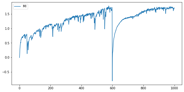
Experiments Sanity check 对于生成数据集进行MI maximization,结果如下
其中我们发现MI在graph中训练时会有sudden collapse的情况。因为是我们人工生成的simulated data,所以还没有办法非常确定这样的现象是不是普遍存在的,是否是MI训练时需要解决的痛点。
Inductive representation learning with InfoGraph Data generation 数据生成的目标还是生成一组unsupervised/train/test数据集。其具体细节我们将略过,其中值得一提的是针对分类问题我们采用了torch中的nn.CrossEntropyLoss这一个损失函数,所以对应生成的标签$Y$应该符合该函数input shape.
Input: $(N, C)$
Target: $(N)$ where each value is $0 \leq \operatorname{targets}[i] \leq C-1$.
Graph Classification Model 该模型作为baseline模型,实现在训练集上的supervised learning. 采用的架构是GCN + SUM_READOUT + Linear + softmax模型.
1 2 3 4 5 6 7 8 9 10 11 12 13 14 15 16 17 18 19 20 21 22 23 24 25 26 27 28 29 30 31 32 33 34 35 36 37 38 39 class GraphClassifier (torch.nn.Module) : def __init__ ( self, d_input=16 , d_hids=(16 , 16 , 16 ) , d_output=16 , dropout=0.2 ) : super(GraphClassifier, self).__init__() self.node_level_model = GCN( d_input=d_input, d_hids=d_hids, d_output=d_output, dropout=dropout ) self.multi_scale_dim = sum(d_hids) + d_output self.classify_model = nn.Sequential( nn.Linear(self.multi_scale_dim, 2 ), nn.Softmax() ) def forward (self, x, adj, y) : multi_scale_node_rep = self.node_level_model(x, adj) node_rep = torch.cat(multi_scale_node_rep, dim=2 ) graph_rep = torch.sum(node_rep, dim=1 , keepdim=False ) y_hat = self.classify_model(graph_rep) criterion = nn.CrossEntropyLoss() loss = criterion(y_hat, y) return y_hat, loss
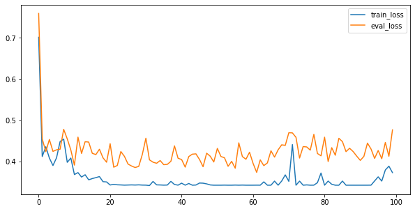
使用该模型进行supervised learning的结果如下
Supervised classifier for representations 1 2 3 4 5 6 7 8 9 10 11 12 13 14 15 16 17 18 19 20 21 class RepClassifier (torch.nn.Module) : def __init__ ( self, d_rep=16 , dropout=0.2 ) : super(RepClassifier, self).__init__() self.classify_model = nn.Sequential( nn.Linear(d_rep, 2 ), nn.Softmax() ) def forward (self, rep, y) : y_hat = self.classify_model(rep) criterion = nn.CrossEntropyLoss() loss = criterion(y_hat, y) return y_hat, loss
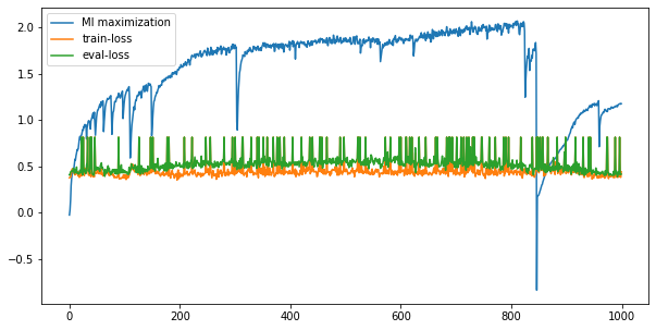
InfoGraph for unsupervised representation learning mi_epoch=10000, cla_epoch=100 , unsup=10000, train=100, test=100
可以看到MI还是会出现sudden collapse的情况。但是从后续representation来看,collapse的发生也并不会导致representation的表现变差。因为test error表现得非常高,所以我们怀疑是否是最后末端加的单层线性加上softmax训练没有拟合。加大cla_epoch的总数,我们有以下结果。
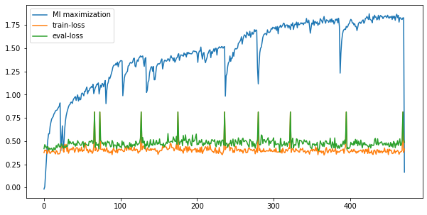
mi_epoch=10000, cla_epoch=500 , unsup=10000, train=100, test=100
我们发现在test上的cross_entropy变得更加稳定,同时当sudden collapse发生的时候对应的eval_loss也会相应地增加。更重要的是,我们发现横坐标并没有一直延伸到10000/10=1000的地方,而是很早就停了下来。打印得到的结果,我们发现后面一半的训练结果是清一色的nan,这也是MI在训练时非常容易达到的状态,或者说是由于我们优化器的选择,超参的选择导致的。
MI在训练时的表现还是需要我们再进一步观察理解,但现在先将在simulated graph data上发现的结果进行一些总结:
MI在maximization的过程中经常会发生sudden collapse,因为是将estimation和maximization同时进行的,这样做会不会带来一些非常糟糕的结果?可能需要参考RL中的estimation.
MI在maximization过程中经常会发生值变为nan的情况,具体原因不明,可能是因为没有采用BN或者weight decay或者采用不适当的优化器(需要进一步调查).