
Materials:
- paper “A Comprehensive Survey on Graph Neural Networks”
- Graph Laplacian Tutorial
- Graph Laplacian explanation on Quora
- Laplacian explanation on Zhihu
- Graph Fourier Transformation Tutorial
- 拉普拉斯算子和拉普拉斯矩阵
- paper “Chebyshev Spectral CNN (ChebNet)”
- paper “Wavelets on Graphs via Spectral Graph Theory”
Notations
Definition 1 (Graph). A graph is represented as $G=(V,E)$, where $V$ is the set of vertices or nodes, and $E$ is the set of edges. In the graph, let $v_i \in V$ to denote a node and $e_{ij}=(v_i, v_j) \in E$ to denote an edge pointing from $v_i$ to $v_j$. (文章中写的是$v_j$ to $v_i$)
Definition 2 (Adjacency matrix & degree matrix). The adjacency matrix $A$ of a graph is a $n\times n$ matrix with
The degree matrix $D$ is a $n\times n$ diagonal matrix with
Lemma 1 (Power of adjacency matrix). Let $G$ be a weighted graph, with binary adjacency matrix $A$. Let $\tilde A$ be the adjacency matrix with unit loops added on every vertex, e.g. $A_{m,n} =\tilde A_{m,n}$ for $m\neq n$ and $\tilde A_{m,n} =1$ for $m=n$. Then for each $s > 0$, $(\tilde A^s)_{m,n}$ equals the number of paths of length s connecting $m$ and $n$, and $(\tilde A^s)_{m,n}$ equals the number of all paths of length $r \leq s$ connecting m and n. (注意:这条引理对于GNN之后推导Locality非常重要)
Definition 3 (Neighborhood of a node). The neighborhood of a node $v$ is defined as
Definition 4 (Node attributes). The node attributes of the graph is represented as $X$, where $X \in \mathbb R ^{n\times d}$ is called as node feature matrix. $x_v \in \mathbb R^d$ represents the feature vector of node $v$.
Definition 5 (Edge attributes). The edge attributes of the graph is represented as $X^e$, where $X^e \in \mathbb R^{m\times c}$ is an edge feature matrix with $x_{v,u}^e ∈ \mathbb R^c$ representing the feature vector of an edge $(v, u)$.
Definition 6 (Spatial-Temporal Graph). A spatial-temporal graph is an attributed graph where the node attributes change dynamically over time. The spatial-temporal graph is defined as $G^{(t)} =(V,E,X^{(t)})$ with $X^{(t)} ∈ \mathbb R^{n\times d}$.
常用的Notation表示一览:
Graph Laplacian
这里我们主要讨论的是undirected graph,对于directed graph来说有其他更多的工作。
How to Define Graph Laplacian?
Definition 7 (Euclidian Laplacian). Laplacian operator in Euclidian space is defined by
Equivalently, the Laplacian of $f$ is the sum of all the unmixed second partial derivatives in the Cartesian coordinates $x_i$:
在欧式空间的拉普拉斯算子就是一个实值函数“梯度的散度”。从物理上来理解拉普拉斯算子的重要性:标量函数的梯度往往是一种“驱动力”(或者叫“势”),而针对“驱动力”求散度就可以知道空间中“源”的分布。
将欧式空间中的Laplacian operator推广到Graph上,需要回答以下几个问题:
- What is the meaning of a function over a graph?
- How do we define the gradient of a graph function?
- How do we define the divergence of the graph gradient?
Graph Laplacian Defintion & Intuition
首先为了定义图函数,我们将图在 $xOy$ 平面上延展开,将节点看成自变量(也就是说节点集合是 $xOy$ 平面上的一个子集),定义函数$ f:V\rightarrow \mathbb R$ 是一个从节点到实数的映射。
接着为了定义图函数上的gradient,回忆起在数值分析中我们学过的difference的概念,也就是在离散空间中梯度的近似近似。同样的我们可以定义:在图上,两个连通节点函数值的difference就是图上的gradient。Gradient of the function along the edge $e=(u,v)$ is given by $\text{grad}(f)|_e=f(u)−f(v)$.
在这个基础上我们先给出graph laplacian的定义:
Definition 8 (Graph Laplacian operator). Graph Laplacian operator $\Delta$ with given graph function $f$ and given node $x$ is defined as
其中$y \sim x$表示节点$y$是$x$的邻接点,也可以表示成$y \in N(x)$. 这条式子定义了一个节点的Laplacian等于该节点所有的incident edge上gradient的和。这就导致了一些疑问:Laplacian是梯度的散度,按照道理应当是gradient的导数的和,为什么这里少了一次求导呢?
为了解决这个疑问,我们回顾在离散空间中的Laplacian是怎样定义的。在一维离散空间上的Laplacian是二阶差分(second-order difference):
而在二维离散空间上的Laplacian算子是矩阵:
该矩阵可以看作是两个正交方向($x$方向和$y$方向)上二阶差分的叠加。通过对比以上的定义,我们需要解决一个问题:如何在graph上计算二阶差分?事实上laplacian在直观上没有办法计算二阶差分,因为在同一个维度(边)上找不到3个节点。为了直观地理解graph laplacian,我们需要重新回到向量场散度的定义。
Definition 9 (Divergence). The divergence of a vector field $F(x)$ at a point $x_0$ is defined as the limit of the ratio of the surface integral of $F$ out of the surface of a closed volume $V$ enclosing $x_0$ to the volume of $V$, as $V$ shrinks to zero.
直观上来讲,散度是计算一点附近邻域内通量的极限。为了将这个概念推广到图结构的离散空间中,我们可以将图结构重新映射到离散的三维空间,我们做以下几个假设:
- 空间中体积的单位元(最小元)是$1\times 1\times 1$的小立方块;
- 图节点是一个单位元;
- 相邻节点有一个面(边)紧贴在一起,在这个面上根据边的梯度定义梯度向量。
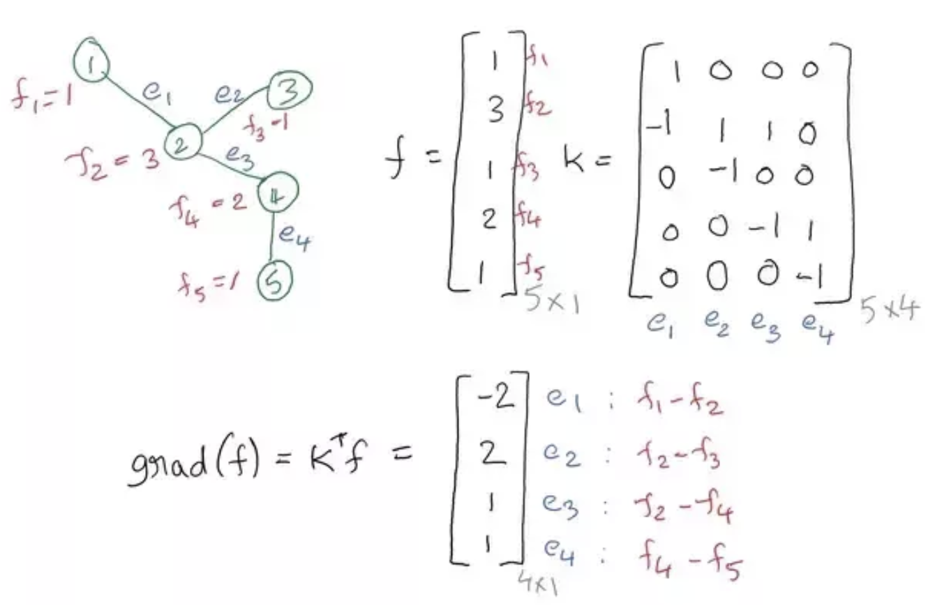
在这个空间中,节点、边、梯度向量场都是离散的。考察具体例子:图$G=(V,E)$以及在图上定义的实值函数 $f:V \rightarrow \mathbb R$,其中$V=\{v_1, v_2, v_3\}$,$E=\{(v_1,v_2), (v_1,v_3)\}$。将这个图映射到我们以上定义的离散空间中,有以下:

该图中的两个箭头表示的梯度向量场分别为 $f(v_1)-f(v_2)$ 以及 $f(v_1)-f(v_3)$. 除此之外的空间中的向量均为$0$向量。那么根据定义,关于节点$v_1$的Laplacian为:
对于更高维度的空间(节点度数$>$8),因为我们认为不同的边是相互正交的,故而也是适用的。从而我们给出了graph laplacian一个更加直观的、符合原定义的解释。
Incidence Matrix
更进一步,我们可以引入关联矩阵(Incidence Matrix)定义一个图函数对于每一条边的gradient:
where $K$ is an $V\times E$ matrix called the incidence matrix. $K$ is constructed as follows: For every edge $e=(u,v)$ in the graph, we assign $K_{u,e}=+1$ and $K_{v,e}=-1$. 我们可以将graph gradient看成是一个新的定义在edge上的函数:$g=\text{grad}(f)$.
关于incidence matrix,有两点需要注意。首先在图论中有一个非常重要的性质:我们认为图上的边相互正交。接着我们可以把一条边看作是空间中的一个维度,所有的边就构成了一个$|E|$维的单位正交基,随意指定维度坐标轴的正向(也就是指定incidence matrix上+1和-1的位置),这样用边集作为基表示的节点集就是incidence matrix.
(注意:graph laplacian可以作为母定义来推导出网格状的二阶差分,但是和网格状的二阶差分相差一个负号)
在graph gradient的基础上定义散度:$\text{div}(g)=Kg$. 而根据定义梯度的散度就是Laplacian,由此我们得到以下定义
Definition 8* (Graph Laplacian operator). Graph Laplacian operator $\Delta$ with given graph function $f$ is defined as
Definition 10 (Standard Graph Laplacian Matrix). Graph Laplacian Matrix $L$ is a $|V|\times |V|$ matrix defined by
where $K$, $A$ and $D$ is the incidence matrix, adjacency matrix and degree matrix respectively of the given graph.
Graph Laplacian和smoothness of graph有一些关联。Dirichlet Energy 定义了图的某种势能,它和variance的定义有些类似:相邻节点的function value应当和他们的edge weight成负相关。Dirichlet Energy可以由Graph Laplacian表示:
在单位球面($f^Tf=1$)上能够minimize Dirichlet energy的 $f$ 就是 $L$ 的smallest nonzero eigenvector。关于这部分的内容在Graph Laplacian explanation on Quora有更多的解释。
Graph Convolution
Definition 11 (Normalized Graph Laplacian Matrix). The normalized graph laplacian matrix $L_n$ is defined as
Lemma 1* (Locality of High Power of Laplacian matrix). Let $G$ be a weighted graph, $L$ the graph Laplacian (normalized or non-normalized) and $s > 0$ an integer. For any two vertices $m$ and $n$, if $d_G(m, n) > s$ then $(L^s)_{m,n} = 0$. 这条引理告诉我们高次的graph laplacian具有高次的局部连通性,具体的证明参考paper “Wavelets on Graphs via Spectral Graph Theory”。
Lemma 2 (Spectral Decomposition). If $A$ is a real symetric matrix, then it can be decomposed as
where $Q$ is an orthogonal matrix whose columns are the eigenvectors of $A$, and $\Lambda$ is a diagonal matrix whose entries are the eigenvalues of $A$.
利用Lemma 2,我们可以将normalized graph Laplacian $L_n$分解为
其中 $U$ 是由$L_n$的特征向量作为列向量构成的$n\times n$方阵,$U$构成了一个orhonormal space,即$U^TU=I$。$\Lambda$是对角元素为$U$对应的特征值的对角阵,$\Lambda$也被称为谱(spectrum)。
Definition 12 (Graph Fourier Transform). The graph Fourier transform is defined by
where $x\in \mathbb R^{|V|}$ is a feature vector (graph signal) of the graph, which means the i-th value of $x$ is the value of the i-th node.
Definition 12* (Inverse Graph Fourier Transform). The inverse graph Fourier transform is defined by
where $\hat x$ is a the result of the graph Fourier transform.
The graph Fourier transform projects the input graph signal to the orthonormal space where the basis is formed by eigenvectors of the nor-malized graph Laplacian.
Definition 13 (Graph Convolution). The graph convolution of the input signal $x$ with a filter $g\in \mathbb R^{|V|}$ is defined as
If we denote a filter as $g_\theta = \text{diag}(U^Tg)$, then the spectral graph convolution is simplified as
所有的Spectral-based ConvGNNs都遵循这个convolution的定义,主要的区别就在于选取不同的filter $g$. 这里我们可以看到,因为$U$是orthonormal basis,所以$U^T$是一个可逆矩阵,也是一个可逆映射。因此当我们参数化$g$的时候可以将这一步矩阵乘法省略,用一个简单的对角矩阵来代替即可。
如果我们将spectrum $\Lambda$作为$g_\theta$的参数,那么我们称满足以下条件的filter称为non-parametric filter,也就是这个filter的自由度就是自身的维度。