Manifold Learning

Basics Manifold

字数统计: 793阅读时长: 3 min

 2020/06/14   Share

Materials

Definition

High-dimensional datasets can be very difficult to visualize. While data in two or three dimensions can be plotted to show the inherent structure of the data, equivalent high-dimensional plots are much less intuitive. To aid visualization of the structure of a dataset, the dimension must be reduced in some way.

Manifold Learning can be thought of as an attempt to generalize linear frameworks like PCA to be sensitive to non-linear structure in data. Though supervised variants exist, the typical manifold learning problem is unsupervised: it learns the high-dimensional structure of the data from the data itself, without the use of predetermined classifications.

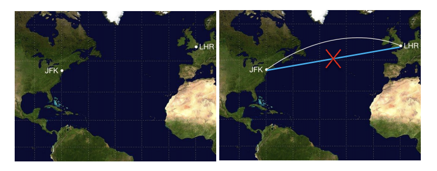
Definition (Geodesic Distance). A geodesic line is the shortest path between two points on a curved surface, like Earth (referring to the following figure).

我认为在Manifold Learning这个领域的最重要假设在于：足够接近的数据点的测地线距离等于他们的欧氏距离。也就是说一小簇点在高维空间可以被看做分布在一个平面上，进而满足线性关系。

Methods

以下方法建立在共同的notation下：我们有一高维数据点集合 $X=\{x_i\}_{i=1}^{N} \sub \mathbb R^D$，现有函数 $f: \mathbb R^D \rightarrow \mathbb R^d$为将高维数据空间映射到表征空间的映射函数，映射后的表征空间$(Y, \rho)$ 是一个欧拉空间，其中：

$\begin{align} Y &=\{y_i\}_{i=1}^{N} \sub \mathbb R^d \\ \rho_{ij} &=\rho(y_i, y_j) = \|y_i-y_j\|_2 \end{align}$

需要注意的是，在Manifold Learning中的$f$经常是没有办法用于新样本的推断的。

Multidimensional Scaling (MDS)

本质上来说，Manifold Learning的学习目标是希望在表征空间上保持整个数据分布的geometry property. 因为我们认为高维数据点在高维空间是分布在一个流型上的，所以距离度量方式并不应当采用欧氏距离，例如如下的优化目标就不合适：

$\min_f\sum_{i,j}(\rho_{ij}-d_{ij})^2$

其中$d_{ij}=d_E(x_i,x_j)$，表示在样本空间的欧氏距离。但基于manifold learning的假设，也就是在一个数据点的很小邻域内，样本间可以近似看作是线性的，因此我们可以只考虑每一个点的邻近点的欧氏距离需要在表征空间中被近似，所以以下的优化目标可以看做保持了样本分布的geometry attributes：

$\min_f \sum_{i=1}^N\sum_{j\sim i}(\rho_{ij}-d_{ij})^2$

以上的优化目标就是MDS的主体部分，它是non-trivial的，虽然我们可以使用梯度下降进行优化。

MDS on dot product

考虑MDS的使用dot product作为度量两个数据点的距离：$K_{ij}=x_i^Tx_j$. 全局优化目标为：

$\min_f \sum_{i,j}(y_i^Ty_j -K_{ij})^2$

于是等价于优化以下目标

$\min \|Y^TY-K\|_F^2$

也就是说MDS在dot product情况下退化成了基于SVD的dimensional reduction method.

$\begin{align} K &= U\Sigma U^T \\ Y &= U_{1:d}\Sigma_{i:d} \end{align}$

Isomap

One of the earliest approaches to manifold learning is the Isomap algorithm, short for Isometric Mapping. Isomap seeks a lower-dimensional embedding which maintains geodesic distances between every two points.

Estimating Geodestic Distance

We could estimate the geodestic distance by constructing an adjacency graph on which the shortest distance between two nodes is the estimation of their geodestic distance. We can set the adjacency matrix following the rule:

$W_{i j}=\left\{\begin{array}{cc} 1 & \left\|x_{i}-x_{j}\right\|<\epsilon \\ 0 & \text { otherwise } \end{array}\right.$

在sklearn主页上，该算法步骤主要由三步构成，第一是为每个点构建Nearest Neighbors，连接这些neighbors就得到了一个在manifold上的连通图；接着需要计算任意两个点之间的geodestic distance；最后使用Partial Eigenvalue Decomposition求得降维后的表示。

Isomap使用 MDS 计算映射后的坐标$y$，使得映射坐标下的欧氏距离与原来的测地线距离尽量相等.

$\min _{f} \sum_{i, j}\left(\rho_{ij} - d_{M}\left(x_{i}, x_{j}\right) \right)^{2}$

Locally Linear Embedding

Locally linear embedding (LLE) seeks a lower-dimensional projection of the data which preserves distances within local neighborhoods. It can be thought of as a series of local Principal Component Analyses which are globally compared to find the best non-linear embedding.

“流形在局部可以近似等价于欧氏空间”是 LLE 分析方法的出发点。LLE认为一个中心数据点 $x_i$ 能够被处于其小邻域内的点$\{x_j\}_{j \sim i}$线性重构，重构的权重可能是我们想要在表征空间上保留的geometry attributes。

$x_i \approx \sum_{j\sim i} W_{ij}x_j$

因而该算法由下面两步构成，首先计算点之间的最优重构权重需要解决以下的优化问题，对$d$维的表征空间，我们需要使用$k\geq d$的kNN来寻找邻接节点。

$\begin{align} &\min_{W}\sum_{i=1}^{N}\left\|x_{i}-\sum_{j \sim i} W_{i j} x_{j}\right\|^{2} \\ &s.t. \sum_{j\sim i}W_{ij}=1,\quad \forall i \in \{1, 2, \cdots, N\} \end{align}$

接着以此作为目标使映射空间中的表征保留该权重，其中对于表征空间上的单位向量的限制是为了防止0向量这个trivial solution.

$\begin{align} \min_Y &\sum_{i=1}^{N} \left\|y_{i}-\sum_{j \sim i} W_{i j} y_{j}\right\|^{2} \\ s.t. &\sum_{i=1}^{N} y_i = 0 \\ & YY^T = I_d \end{align}$